Table of Contents:
Introduction:
Sample:
Report:
Plot:
Database:
Options:
Cropping:
Scan Diagnostics:
Computer Specifications:
Glossary:
Introduction:
 The
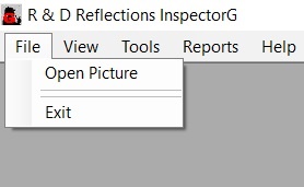
basic operation of the InspectorG software is very simple and once it is
configured to display the desired parameters, it can be used after just a few
minutes of instruction. The first step is to open an image from the "File" menu
as shown here. This will open a dialog window that defaults to the last folder
used. It will normally contain a selection of images that are to be analyzed,
but in some cases it will be necessary to change folders to locate the images
that have been previously stored. If you are starting from a new installation
and wish to use the sample images that are provided they will be found in a
folder C:\Users\Public\Public Documents\R & D Reflections\InspectorG\Samples.
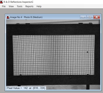
Opening an image will present an image such as that below. It is possible to
have multiple unanalyzed pictures open on the screen at the same time. Each
picture is identified by its original name and an Image No that is the sequence
in which they have been opened. Only the select picture will be processed when
an analysis is started.
The
basic operation of the InspectorG software is very simple and once it is
configured to display the desired parameters, it can be used after just a few
minutes of instruction. The first step is to open an image from the "File" menu
as shown here. This will open a dialog window that defaults to the last folder
used. It will normally contain a selection of images that are to be analyzed,
but in some cases it will be necessary to change folders to locate the images
that have been previously stored. If you are starting from a new installation
and wish to use the sample images that are provided they will be found in a
folder C:\Users\Public\Public Documents\R & D Reflections\InspectorG\Samples.
Opening an image will present an image such as that below. It is possible to
have multiple unanalyzed pictures open on the screen at the same time. Each
picture is identified by its original name and an Image No that is the sequence
in which they have been opened. Only the select picture will be processed when
an analysis is started.
 In most
instances, the system is ready to proceed with the analysis at this point. The
software is designed to automatically locate the outline of the sample but in a
few cases this may fail and the region of interest will need to be selected with
the mouse (cropped). This is done by selecting one corner of the grid and
holding the left mouse button down, then dragging the mouse to the opposite
corner and releasing. The cropped outline may be adjusted with the mouse by
clicking on an edge or corner and dragging to the correct position. Partial
regions of the image may also be selected in this way. More details about
cropping will be described later.
In most
instances, the system is ready to proceed with the analysis at this point. The
software is designed to automatically locate the outline of the sample but in a
few cases this may fail and the region of interest will need to be selected with
the mouse (cropped). This is done by selecting one corner of the grid and
holding the left mouse button down, then dragging the mouse to the opposite
corner and releasing. The cropped outline may be adjusted with the mouse by
clicking on an edge or corner and dragging to the correct position. Partial
regions of the image may also be selected in this way. More details about
cropping will be described later.
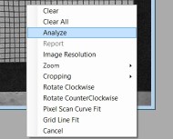
One item to note is the message that appears in the lower left border of the picture. This provides the gray scale value of the pixel where the mouse is currently pointed. This information is not needed to operate and use the software to produce numerical values for the distortion of a sample. It can, however, be useful for a full understanding of how the analysis is done and for understanding some of the diagnostic tools that will be described later. Each image is really just a collection of numbers that represent the brightness of each point in the picture. Each point can be a value that ranges from 0 (Black) to 255 (White) with most being intermediate (grayscale). The co-ordinate system describes each point in the picture as a value X, the distance from the left edge, and Y the distance down from the top of the picture. It is now time to analyze the sample, which can be done from the main top "Tools" menu, or easier by right-clicking on the image which brings up the following context menu. Simply, click on the analyze selection and the process will begin.
 If you
have chosen to add customized information to each sample run, a window will open
that allows the selection and entering of this information. Details of this will
be provided later in the Custom Fields section. If not, the analysis will
proceed and its progress is indicated by a series of yellow dots that overlay
the black grid lines in the original image. If there is any problem fitting the
grid lines, the progression of yellow dots will pause or not cover the entire
image area. At the completion of the analysis a number of things will happen. A
report form will open in the lower right area of the screen which will display
some of the most important results. Also, the yellow lines in the image will now
be overwritten with a grid of red lines that display the shape of the mathematical
grid that has been fitted. Additionally, all data that has been calculated is
entered into the database and displayed in the database window. Finally, a
surface plot of the appropriate distortion pattern is opened if the "autoplot"
selection is checked in the "Tools-Option" menu. Each of these items will be
described in detail in their specific section. This completes the analysis of a
selected image and all that remains is to understand and interpret the results
and learn how to configure the few options available. An option is provided to
rotate an image before analysis. This is useful to orient the conveyence
direction to be horizontal when in the roll wave mode.
If you
have chosen to add customized information to each sample run, a window will open
that allows the selection and entering of this information. Details of this will
be provided later in the Custom Fields section. If not, the analysis will
proceed and its progress is indicated by a series of yellow dots that overlay
the black grid lines in the original image. If there is any problem fitting the
grid lines, the progression of yellow dots will pause or not cover the entire
image area. At the completion of the analysis a number of things will happen. A
report form will open in the lower right area of the screen which will display
some of the most important results. Also, the yellow lines in the image will now
be overwritten with a grid of red lines that display the shape of the mathematical
grid that has been fitted. Additionally, all data that has been calculated is
entered into the database and displayed in the database window. Finally, a
surface plot of the appropriate distortion pattern is opened if the "autoplot"
selection is checked in the "Tools-Option" menu. Each of these items will be
described in detail in their specific section. This completes the analysis of a
selected image and all that remains is to understand and interpret the results
and learn how to configure the few options available. An option is provided to
rotate an image before analysis. This is useful to orient the conveyence
direction to be horizontal when in the roll wave mode.
Sample:
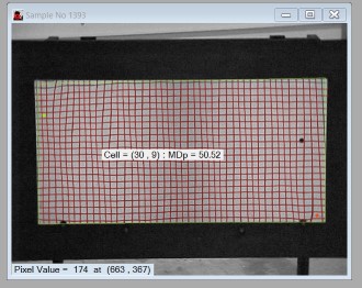 The final
view of the sample at the conclusion of the analysis is illustrated here. You
can see the red grid overlay that should cover the entire area that was
originally selected. The outline is shown in green and this is either the
auto-detected outline or the selected crop region. The display in the center of
the grid shows the millidiopter value at the cell location of the mouse pointer.
The cells are numbered from left to right and top down in the same way the
individual pixel points are numbered. This value will only be available for
completely enclosed cells that have been evaluated so this is a good method to
see that the analysis is completed for the entire sample.
The final
view of the sample at the conclusion of the analysis is illustrated here. You
can see the red grid overlay that should cover the entire area that was
originally selected. The outline is shown in green and this is either the
auto-detected outline or the selected crop region. The display in the center of
the grid shows the millidiopter value at the cell location of the mouse pointer.
The cells are numbered from left to right and top down in the same way the
individual pixel points are numbered. This value will only be available for
completely enclosed cells that have been evaluated so this is a good method to
see that the analysis is completed for the entire sample.
Two other items to note are the red dot in the lower right and the green dot in the upper left position. These locations mark the largest and smallest cell area and consequently the largest and smallest millidiopter value for the sample. Although both optical power and rollwave millidiopters are calculated for all samples, only one of these is displayed on the sample. The mode displayed is determined by which tab is selected in the report form. Also, when rollwave is selected the maximum and minimum cells are highlighted by orange and blue dots rather than the red and green dots of the optical power mode. If any of the results in the report form or on the database form appear suspicious in any way, this window is an excellent place to look for errors in the grid fitting process. Errors that prevent tracing the lines in some areas may appear as red lines that do not follow the original black grid lines of the photo. The most common issues here might be lighting that cause low contrast areas or other such defects in the original image.
Report:
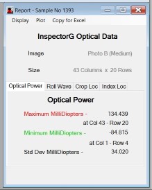 The report window
collects the most important results of the analysis into one concise
summary of the extensive evaluations that have been performed. The report shown
here is for optical power as seen by the highlighted tab in the center of the
window, but most of this discussion also applies to the rollwave mode. The
report shows the name of the original image file that began the process and also
the number of cells found in the rectangular array. The region at the bottom of
the report provides the most important numbers that characterize a specific
sample. Some people emphasize the worst value as the determinant of overall
quality. The standard deviation, however, is a statistical representation of the
overall distortion level of the sample, and may be a better number to classify a
sample. This is a decision that each user must make for their own best
utilization of this tool.
The report window
collects the most important results of the analysis into one concise
summary of the extensive evaluations that have been performed. The report shown
here is for optical power as seen by the highlighted tab in the center of the
window, but most of this discussion also applies to the rollwave mode. The
report shows the name of the original image file that began the process and also
the number of cells found in the rectangular array. The region at the bottom of
the report provides the most important numbers that characterize a specific
sample. Some people emphasize the worst value as the determinant of overall
quality. The standard deviation, however, is a statistical representation of the
overall distortion level of the sample, and may be a better number to classify a
sample. This is a decision that each user must make for their own best
utilization of this tool.
There are two additional tab positions on the report form that provide additional information about each sample. The first captures any cropping position for the situation where a comparison needs to be made between two or more samples, and the same region needs to be used for all. The last tab on this form records the cell location of an index mark which is a single solid black cell in the middle of the grid. At this time, this is only used when transmitted distortion is measured as it is required to properly overlay a test image over an image of the grid with no sample(calibration).
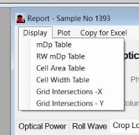 The three menu selections at the top of the report form allow very detailed
information about a sample to be viewed and also exported to an Excel spread
sheet if any additional calculations are desired. The first selection presents a
tabular view of the listed items for each cell in the sample. Virtually all of
the measurements made during the analysis are available in one of these
displays. The third menu item provides a means for these same display tables to
be pasted into an Excel spread sheet. The center menu provides for plotting both
optical power millidiopters and rollwave millidiopter values on a colored
surface-like plot. If the auto-plot option has been selected in the main window
menu the appropriate plot is shown at the completion of the analysis when the
report is opened. This "Plot" menu will allow viewing a plot of the mode not
selected in the tabs.
The three menu selections at the top of the report form allow very detailed
information about a sample to be viewed and also exported to an Excel spread
sheet if any additional calculations are desired. The first selection presents a
tabular view of the listed items for each cell in the sample. Virtually all of
the measurements made during the analysis are available in one of these
displays. The third menu item provides a means for these same display tables to
be pasted into an Excel spread sheet. The center menu provides for plotting both
optical power millidiopters and rollwave millidiopter values on a colored
surface-like plot. If the auto-plot option has been selected in the main window
menu the appropriate plot is shown at the completion of the analysis when the
report is opened. This "Plot" menu will allow viewing a plot of the mode not
selected in the tabs.
Note that the report form may be reopened through the right-click menu of the sample window if it has been closed.
Plot:
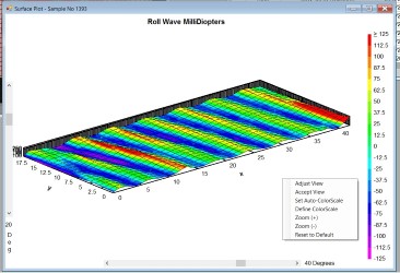 The plot window is
mostly self explanatary, but there are a number of choices available for
configuring the desired appearance. Right-clicking anyplace in the plot window
will display a menu list as shown in the picture. Selecting the first menu item
"Adjust View" will display the vertical and horizontal scroll bars shown at
left. These can be moved with the mouse to adjust the orientation of the plot.
If a new viewpoint is found to be better it can be saved as the default view.
The color scale can also be defined so that the red and violet extremes
represent a fixed numeric value. This may be best for the comparison of plots
between different samples. This setting may also be selected as "Auto" in which
case the extreme colors are defined as plus or minus two times the standard
deviation. This setting is most appropriate when samples with wildly different
distortion are being processed. The last adjustment is called zoom and it
modifies the 3-D effect of the plot by stretching the vertical Z-axis. It is
important to remember that this is not really a surface representation but
merely a visual aid for viewing the optical distortion distribution.
The plot window is
mostly self explanatary, but there are a number of choices available for
configuring the desired appearance. Right-clicking anyplace in the plot window
will display a menu list as shown in the picture. Selecting the first menu item
"Adjust View" will display the vertical and horizontal scroll bars shown at
left. These can be moved with the mouse to adjust the orientation of the plot.
If a new viewpoint is found to be better it can be saved as the default view.
The color scale can also be defined so that the red and violet extremes
represent a fixed numeric value. This may be best for the comparison of plots
between different samples. This setting may also be selected as "Auto" in which
case the extreme colors are defined as plus or minus two times the standard
deviation. This setting is most appropriate when samples with wildly different
distortion are being processed. The last adjustment is called zoom and it
modifies the 3-D effect of the plot by stretching the vertical Z-axis. It is
important to remember that this is not really a surface representation but
merely a visual aid for viewing the optical distortion distribution.
Database:
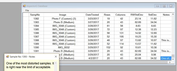 The database
window is always present and maintains a full history of the samples tested with
this software. This window is a very flexible viewpoint into the calculation
results that are all stored in a SQL database called SQLite. This is a very
common, fast, and well documented piece of open source software. The user has
complete control over which variables are displayed from a selection made in the
"Tools-Option" menu on the main window. The columns can be ordered in any way
and the rows can also be sorted in either direction based on the content of a
specific column by clicking on that column's heading. One feature shown in this
window is a special field called notes that is not an analysis result. Instead,
it may be entered at the time of processing but is the only field in the
database that can be edited later. This allows retaining any specific
information that may be seen as a result of examining the data. Clicking on this
note field opens a small window as shown for editing.
The database
window is always present and maintains a full history of the samples tested with
this software. This window is a very flexible viewpoint into the calculation
results that are all stored in a SQL database called SQLite. This is a very
common, fast, and well documented piece of open source software. The user has
complete control over which variables are displayed from a selection made in the
"Tools-Option" menu on the main window. The columns can be ordered in any way
and the rows can also be sorted in either direction based on the content of a
specific column by clicking on that column's heading. One feature shown in this
window is a special field called notes that is not an analysis result. Instead,
it may be entered at the time of processing but is the only field in the
database that can be edited later. This allows retaining any specific
information that may be seen as a result of examining the data. Clicking on this
note field opens a small window as shown for editing.
Finally, a very important feature of this database window is the ability to retrive not only the tabular data, but the image of the sample, the associated report form, and also the distortion plot. This means that any historical sample may be totally reviewed exactly as if newly analyzed. This is accomplished simply by clicking on any cell in the database window.
Options:
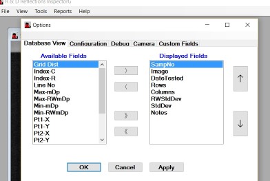 The final
significant and frequently used form is the "Options" window that is displayed
from either the "View" or "Tools" menu on the main screen. This is where most of
the customization is done to configure the visual expression or the actual
performance of the InspectorG software. The first tab offers a selection list of
the fields that are displayed in the database window. Every variable that
results from the sample analysis is shown here in either the diplayed or
available list. Two actions are available here to move variables back and forth
between these two lists. Either select a variable and then click the appropriate
directional arrow or simply double click a variable in either list and it will
move to the other. In addition, the order of display in the database form is
determined by the order of display in the displayed field list. The vertical
arrow buttons are used to re-order the columns displayed in the database. The
database window display is updated to reflect these changes whenever the "OK" or
"Apply" button is clicked.
The final
significant and frequently used form is the "Options" window that is displayed
from either the "View" or "Tools" menu on the main screen. This is where most of
the customization is done to configure the visual expression or the actual
performance of the InspectorG software. The first tab offers a selection list of
the fields that are displayed in the database window. Every variable that
results from the sample analysis is shown here in either the diplayed or
available list. Two actions are available here to move variables back and forth
between these two lists. Either select a variable and then click the appropriate
directional arrow or simply double click a variable in either list and it will
move to the other. In addition, the order of display in the database form is
determined by the order of display in the displayed field list. The vertical
arrow buttons are used to re-order the columns displayed in the database. The
database window display is updated to reflect these changes whenever the "OK" or
"Apply" button is clicked.
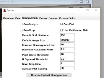 The
configuration tab lists a number of variables that can be changed to affect the
internal operations of the software analysis. Most of these will not be useful
to modify as they are tuned to achieve best robustness in the search algorythms.
The only variable likely to be changed is the Grid Distance that should
acurately reflect the geometry of the inspection station. Each will be defined in
the glossary list below. The checkboxes at the top are more frequently changed
to suit the desired behavior of the analysis and display.
The
configuration tab lists a number of variables that can be changed to affect the
internal operations of the software analysis. Most of these will not be useful
to modify as they are tuned to achieve best robustness in the search algorythms.
The only variable likely to be changed is the Grid Distance that should
acurately reflect the geometry of the inspection station. Each will be defined in
the glossary list below. The checkboxes at the top are more frequently changed
to suit the desired behavior of the analysis and display.
The third tab on the options page contains a few debug checkboxes that select timing or sequence reports that may be helpful to diagnose sample dependent or other operational problems. These are not intended as user tools but may be requested by the developers to solve site developed issues.
The next tab is marked "Camera" and is not used at this time. It is under development to contain geometrical parameters that define the camera location and direction of view. These parameters will be determined by a calibration proceedure and will then be used to correct the image for misalignmet of the camera from the desired perpendicular view. It will also contain correction factors for the particular camera lens in use to improve the image accuracy.
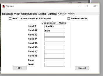 The fimal tab labeled "Custom Fields"
provides a method for the user to add customized information to the database
that is not directly calculated by the software. To use this, a description-name
of the additional information is entered on this form. Up to ten additional
items may be added to the database from this form although most situations will
only require a small number of them. This information will be unique to the way
the software is used at each installation. Since the software will not be aware
of this information, it will need to be entered manually for each sample at the
time of analysis. As an example, a plant with multiple production lines might
want to record which line produced a particular sample. In this case, "Line No"
is entered on the Field # 1 line in this form. When the sample is analyzed, a
small window will open to prompt the user for this information. If you look
above at the database view window you can see that "Line No" is one of the
available fields to select for display in the database window. It is optional to
use this additional information and the feature may easily be disabled by
unchecking the box at the top of this form. The "Note" field may also be
included at this time if desired, or it may be reseved for later use only after
the analysis is completed.
The fimal tab labeled "Custom Fields"
provides a method for the user to add customized information to the database
that is not directly calculated by the software. To use this, a description-name
of the additional information is entered on this form. Up to ten additional
items may be added to the database from this form although most situations will
only require a small number of them. This information will be unique to the way
the software is used at each installation. Since the software will not be aware
of this information, it will need to be entered manually for each sample at the
time of analysis. As an example, a plant with multiple production lines might
want to record which line produced a particular sample. In this case, "Line No"
is entered on the Field # 1 line in this form. When the sample is analyzed, a
small window will open to prompt the user for this information. If you look
above at the database view window you can see that "Line No" is one of the
available fields to select for display in the database window. It is optional to
use this additional information and the feature may easily be disabled by
unchecking the box at the top of this form. The "Note" field may also be
included at this time if desired, or it may be reseved for later use only after
the analysis is completed.
Cropping:
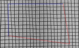 The
cropping feature can be anything from a very simple rectangular outline used
one time to select a region of interest on a sample before triggering the
analysis, to a more complicated action of selecting one of five previously
saved shapes. The simple method only requires holding the mouse left button
down while dragging the mouse to an opposite corner. A slightly more complex
outline can be created by subsequently depressing the left mouse button
while hovering over one of the existing corners and dragging it to a new
position. This allows irregular shapped outlines for the selected region
with the only limit being a four sided shape. Some limitations exist on the
complesity for the analysis but it can handle most reasonable shapes that may
not be perfectly aligned with the edges. Note that the edges turn from blue
to red to indicate when the mouse is within the selection tolerence.
The
cropping feature can be anything from a very simple rectangular outline used
one time to select a region of interest on a sample before triggering the
analysis, to a more complicated action of selecting one of five previously
saved shapes. The simple method only requires holding the mouse left button
down while dragging the mouse to an opposite corner. A slightly more complex
outline can be created by subsequently depressing the left mouse button
while hovering over one of the existing corners and dragging it to a new
position. This allows irregular shapped outlines for the selected region
with the only limit being a four sided shape. Some limitations exist on the
complesity for the analysis but it can handle most reasonable shapes that may
not be perfectly aligned with the edges. Note that the edges turn from blue
to red to indicate when the mouse is within the selection tolerence.
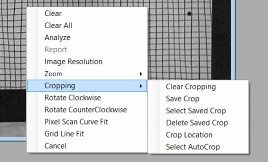 The extended
cropping features are reached by right-clicking anywhere on the sample image
which will open the context menu shown here. A secondary click on the
"Cropping" item will then open the submenu also shown in this picture. In
this menu it is possible to save the previously selected crop outline, with
a limit of five saved shapes. This is useful when a specific subarea is to
be compared on a series of samples. Another obvious functions on this menu
is "Clear" to erase the existing crop. Although five different regions may
be saved at one time, one of these has a special designation as the
"AutoCrop". This is either the last one saved or it may be graphically
selected from the various saved regions with the mouse. This "AutoCrop"
shape is outlined in yellow with the rest in an orange color. This is the
region selected when the "AutoCrop" option is selected in the main window
"Options" menu.
The extended
cropping features are reached by right-clicking anywhere on the sample image
which will open the context menu shown here. A secondary click on the
"Cropping" item will then open the submenu also shown in this picture. In
this menu it is possible to save the previously selected crop outline, with
a limit of five saved shapes. This is useful when a specific subarea is to
be compared on a series of samples. Another obvious functions on this menu
is "Clear" to erase the existing crop. Although five different regions may
be saved at one time, one of these has a special designation as the
"AutoCrop". This is either the last one saved or it may be graphically
selected from the various saved regions with the mouse. This "AutoCrop"
shape is outlined in yellow with the rest in an orange color. This is the
region selected when the "AutoCrop" option is selected in the main window
"Options" menu.
Scan Diagnostics:
 The
two tools described in this section are definately not required for a basic
understanding of the operation of InspectorG, but for those who would like
to have a better understanding of the methods behind the scene they can be
very interesting. The Pixel line fit represents the action of finding a list
of points that makeup a gridline, then fitting a multisegment cubic spline
to these points, and plotting this curve. The particular grid line depicted
is the first vertical one to the right of the point X=499, Y=434.
Approximately 350 points are collected along this line and they are shown as
red dots in the plot. Each of these points is listed in the listbox just to
the left of the "Outline" button. The Segments textbox indicates that 23
spline segments are used to best fit these points. At the far right side is
a list of the 23 cubic spline parameters. From those 72 parameters an exact
mathematical equation is produced that gives the X location of every pixel
along this line. The thin blue line almost hidden behind the red dots is a
curve plot of this spline. The primary purpose of these tools was to test the
mathematics underlying the overall analysis. The exact same routines are
used in these tools as in the main system. Now, they provide an excellent
testing approach if the main system runs into problems. With this form the
entire sample image can be scanned line by line using the "Next" and
"Previous Line" buttons.
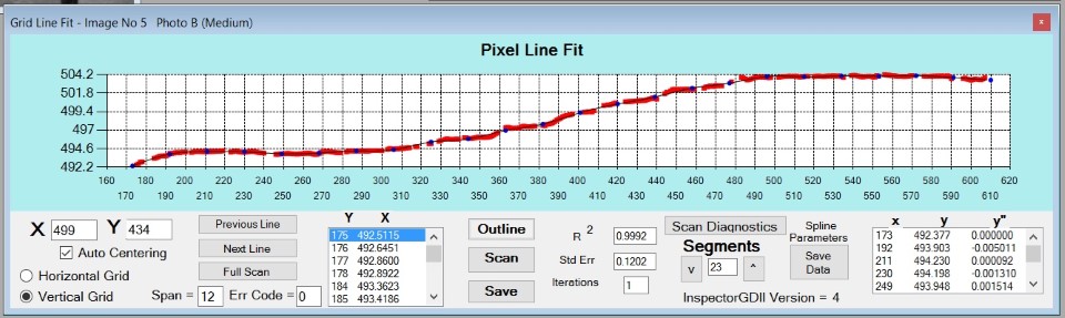
The
two tools described in this section are definately not required for a basic
understanding of the operation of InspectorG, but for those who would like
to have a better understanding of the methods behind the scene they can be
very interesting. The Pixel line fit represents the action of finding a list
of points that makeup a gridline, then fitting a multisegment cubic spline
to these points, and plotting this curve. The particular grid line depicted
is the first vertical one to the right of the point X=499, Y=434.
Approximately 350 points are collected along this line and they are shown as
red dots in the plot. Each of these points is listed in the listbox just to
the left of the "Outline" button. The Segments textbox indicates that 23
spline segments are used to best fit these points. At the far right side is
a list of the 23 cubic spline parameters. From those 72 parameters an exact
mathematical equation is produced that gives the X location of every pixel
along this line. The thin blue line almost hidden behind the red dots is a
curve plot of this spline. The primary purpose of these tools was to test the
mathematics underlying the overall analysis. The exact same routines are
used in these tools as in the main system. Now, they provide an excellent
testing approach if the main system runs into problems. With this form the
entire sample image can be scanned line by line using the "Next" and
"Previous Line" buttons.
 The form to the left
illustrates the method for determining each point along the gridline described above.
For each horizontal line of pixels that cross a vertical grid line the 12
grey scale values centered about it are read from the original image file.
These are shown here by the red dots in the plot. The physical meaning of
these points show a nearly white background at the two ends of the curve,
and four or five points near the middle that approach black in the middle.
The greyscale values are shown in the "Y Values" listbox. A mathematical
Gaussian function is fit to these points and the R-Squared statistical
measure of fit is .98 indicating a very good data fit. Using the center
value of the curve, "C" in the parameters, the center of this gridline is
evaluated to be 492.51, the 487 X value is the starting point for the scan.
This is the method that allows the center of a grid line to be measured much
more accurately than the smallest piece of data (the pixel). One of these
scans is made for each line of pixels from the top to bottom of the image
and each point is entered into the linefit curve described above. When an
image is questionable because of low contrast or lighting this screen can be
stepped around the image with the 4 directional buttons to find areas where
good fits are not possible. Values for the grid line center are rejected
when the Gaussian fit is below a certain statistical value and the return
code is not valid.
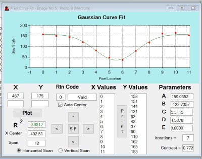
The form to the left
illustrates the method for determining each point along the gridline described above.
For each horizontal line of pixels that cross a vertical grid line the 12
grey scale values centered about it are read from the original image file.
These are shown here by the red dots in the plot. The physical meaning of
these points show a nearly white background at the two ends of the curve,
and four or five points near the middle that approach black in the middle.
The greyscale values are shown in the "Y Values" listbox. A mathematical
Gaussian function is fit to these points and the R-Squared statistical
measure of fit is .98 indicating a very good data fit. Using the center
value of the curve, "C" in the parameters, the center of this gridline is
evaluated to be 492.51, the 487 X value is the starting point for the scan.
This is the method that allows the center of a grid line to be measured much
more accurately than the smallest piece of data (the pixel). One of these
scans is made for each line of pixels from the top to bottom of the image
and each point is entered into the linefit curve described above. When an
image is questionable because of low contrast or lighting this screen can be
stepped around the image with the 4 directional buttons to find areas where
good fits are not possible. Values for the grid line center are rejected
when the Gaussian fit is below a certain statistical value and the return
code is not valid.
Computer Specifications:
InspectorG is written to operate on a Windows 10 based computer. It should operate on mid-range standard hardware with no special requirements on the video display performance. The images and gridline data are stored for each sample tested but memory requirements should not be inordinately high for most use. If using a grid with small cells and large sample sizes, the processing effort will be high and the best performing computer will be a good investment.
Glossary:
- Accept View:
- Makes the current plot view the default.
- Adjust View:
- Allows elevation and azimuth adjustment of the surface plot viewpoint.
- AutoAnalyze:
- A checkbox in the main "Options" menu that triggers analysis immediately after an image is selected.
- AutoCrop:
- A checkbox in the main "Options" menu that loads the autocrop region, if one is designated, immediately after an image is selected.
- AutoPlot:
- A checkbox in the main "Options" menu that triggers a surface plot immediately after an analysis is completed.
- Calibration Grid:
- An image made of a gridboard with no distorting sample, that is used to improve accuracy of samples by comparison.
- Cell:
- A localized area on an image or gridboard, usually square that is between adjacent vertical and horizontal gridlines.
- Columns:
- In the database - the number of columns in the analyzed region.
- Custom Fields:
- User defined and entered data for each sample.
- DataLog:
- A text file that logs all sample runs and contains the same information as the database. C:\User\Public\Public Documents\R & D Reflections\InspectorG\Data\Datafile.txt.
- Date Tested:
- The Date of sample analysis.
- Default Image Size:
- A configuration setting that specifies the size of a newly loaded image in pixels.
- Define ColorScale:
- Allows uset definition of plot color scaling.
- DplotJr:
- A third party plotting software used to display the surface mappings. This is installed with InspectorG and is available as a stand alone program, but is transparent to user.
- Grid:
- A complete pattern of vertical and horizontal gridlines(gridboard).
- Grid Dist:
- The physical distance from the camera to the sample, and also from the sample to the gridboard - approximately 4 meters.
- Gridline:
- A single black line on a gridboard or in the reflected image.
- Image:
- A general term for the digital picture of the sample reflected in the gridboard.
- Index:
- A central cell(black) on a gridboard that creates a mark on an image for positioning an image overlay.
- Index-C:
- The column number of a special black marker cell in a calibration grid image, measured from the left side.
- Index-R:
- The row number of a special black marker cell in a calibration grid image, measured from the top.
- Iteration Convergence Limit:
- The maximum attempts in fitting a Gaussian curve to pixel scan data. Not intended as a user setting.
- Max-mDp:
- The value of largest positive mDp over the surface of an analyzed sample.
- Max-RWmDp:
- The value of largest positive RWmDp over the surface of an analyzed sample.
- mDp:
- A physical unit abreviation for milliDiopter - related to lens power and curvature.
- A specific value applied to a location(cell) that represents the local "Optical Power"
- Maximum Gaussian Width:
- A limit on the Gaussian width parameter used to filter poorly fitting gridline data. Not intended as a user setting.
- Min-mDp:
- The value of largest negative mDp over the surface of an analyzed sample.
- Min-RWmDp:
- The value of largest negative RWmDp over the surface of an analyzed sample.
- Pixel:
- A single spot on a digital image that indicates it's whiteness (0-255), or multipe color levels on a color image.
- Pixel White Threshold:
- A minimum limit on the "white" level of the Gaussian pixel data used to filter very dark image areas. Not intended as a user setting.
- Pt1-X:
- The X pixel position of the upper left point on a cropped region or of the outlined region(measured from left side).2
- Pt1-Y:
- The Y pixel position of the upper left point on a cropped region or of the outlined region(measured from top).
- Pt2-X:
- The X pixel position of the upper right point on a cropped region or of the outlined region(measured from left side).
- Pt2-Y:
- The Y pixel position of the upper right point on a cropped region or of the outlined region(measured from top).
- Pt3-X:
- The X pixel position of the lower right point on a cropped region or of the outlined region(measured from left side).
- Pt3-Y:
- The Y pixel position of the lower right point on a cropped region or of the outlined region(measured from top).
- Pt4-X:
- The X pixel position of the lower left point on a cropped region or of the outlined region(measured from left side).
- Pt4-Y:
- The Y pixel position of the lower left point on a cropped region or of the outlined region(measured from top).
- Rollwave:
- A roughly sinesoidal shape that is characteristic of glass tempered on a roll bed tempering furnace.
- Rows:
- In the database - the number of rows in the analyzed region.
- R Squared Threshold:
- A minimum limit on the statistical Gaussian curve fit to the pixel data. Not intended as a user setting.
- RW mDp:
- A specific value applied to a location(cell) - related to local cylindrical curvature.
- RWStdDev:
- The statistical standard deviation of all of the RWmDp values in a sample.
- Sample:
- The physical object tested.
- The window that shows the grid image.
- The row in the database form that contains all results after analysis.
- Sample No:
- A unique number that always represents a sample and its analysis result.
- Scan Step Size:
- The increment step for Gaussian cross scans along a gridline. Also, an increment for skipping gridlines in a grid scan. A variable intended to decrease time for an analysis (usually 1).
- Set Auto-ColorScale:
- Allows software to establish maximum color milliDiopter values at two times standard deviation.
- StdDev:
- The statistical standard deviation of all of the mDp values in a sample.
- Surface Plot Scaling:
- The milliDiopter value indicated by the extreme colors (red) for the plot legend.
- TimeofTest:
- The time of sample analysis.
- In the database - the computer file name of an image.
- Use Calibration Grid:
- A checkbox in the main "Options" menu that corrects an image by comparison with a calibration image. At present this only applies to transmitted mode.
- Zoom:
- User adjustment of 3-D effect in surface plot.